chaidr

chaidr is a base R implementation of the CHAID (Chi-squared Automatic Interaction Detection) and Exhaustive CHAID decision tree algorithms, as specified in the IBM SPSS Statistics Algorithms documentation (Kass 1980; Biggs, de Ville, and Suen 1991). The core fitting and prediction routines depend only on base R – visualization backends and ‘partykit’ integration are optional soft dependencies.

日本語版 README は README.ja.md を参照してください。

Features

• Standard CHAID and Exhaustive CHAID tree growing with multi-way splits.
• Predictors: nominal, ordinal (with a floating category for missing values), and continuous (automatically discretized into quantile bins).
• Responses: nominal (Pearson chi-squared test), ordinal (Goodman row-effects model), and continuous (one-way ANOVA F test).
• Frequency weights via freq, reproducing results on pre-aggregated data.
• Prediction of classes, class probabilities, and node membership with predict().
• Model inspection: node tables (chaid_table()), decision rules (chaid_rules()), and predictor importance (chaid_importance()).
• Evaluation: gains and lift analysis (chaid_gains()) and validation on holdout data (chaid_validate()).
• Visualization: base graphics plot(), ‘Graphviz’ DOT export (chaid_dot(), chaid_graphviz()), interactive ‘plotly’ trees (chaid_plotly()), and conversion to ‘partykit’ objects (chaid_as_party()).

When to use CHAID

If predictive accuracy is the only goal, modern gradient-boosting methods such as ‘XGBoost’ and ‘LightGBM’ will usually outperform CHAID. CHAID’s strengths lie elsewhere: interpretability of the results, direct connection to decision making, and statistical justification for every split. Rather than a black box, CHAID builds a single multi-way tree in which each split is backed by a significance test, which is why it remains a strong choice in consulting and marketing practice.

Typical applications:

• Survey analysis, customer-satisfaction (CS) studies, and market research
• Marketing segmentation and target selection
• Domains with strong accountability requirements, where every decision rule must be explainable
• Early-stage exploratory data analysis (EDA)

Installation

Once on CRAN, install the released version with:

install.packages("chaidr")

Until then, you can install the development version from GitHub:

# install.packages("remotes")
remotes::install_github("morimotoosamu/chaidr")

Quick start

The penguins data set (bundled with R >= 4.5) contains a mix of continuous predictors and missing values, both of which CHAID handles natively.

library(chaidr)

data(penguins)
fit <- chaid(species ~ ., data = penguins,
             control = chaid_control(min_parent = 30, min_child = 10))
print(fit)
#> CHAID decision tree (method = "chaid")
#> Response: species (categorical) 
#> Valid cases: 344 (data: 344 rows) 
#> 
#> [1] root: Adelie (44.2%), n=344 | split: flipper_len (adj.p=2.48e-63, chi2=328.5, B=714)
#>   [2] flipper_len in {<= 190}: Adelie (84.8%), n=99 | split: bill_len (adj.p=2.92e-16, chi2=78.21, B=28)
#>     [3] bill_len in {<= 40.1}: Adelie (100.0%), n=70 *
#>     [4] bill_len in {(40.1, 41.8]}: Adelie (92.3%), n=13 *
#>     [5] bill_len in {(41.8, 47.3] | > 49.3}: Chinstrap (87.5%), n=16 *
#>   [6] flipper_len in {(190, 196]}: Adelie (67.2%), n=67 | split: bill_len (adj.p=1.66e-13, chi2=58.69, B=9)
#>     [7] bill_len in {<= 44.4}: Adelie (100.0%), n=43 *
#>     [8] bill_len in {> 44.4}: Chinstrap (91.7%), n=24 *
#>   [9] flipper_len in {(196, 202]}: Chinstrap (52.6%), n=38 | split: bill_len (adj.p=2.31e-07, chi2=30.78, B=8)
#>     [10] bill_len in {<= 45.9}: Adelie (90.0%), n=20 *
#>     [11] bill_len in {> 47.3}: Chinstrap (100.0%), n=18 *
#>   [12] flipper_len in {(202, 214] | <NA>}: Gentoo (73.8%), n=61 | split: bill_dep (adj.p=9.69e-12, chi2=56.14, B=15)
#>     [13] bill_dep in {<= 16.7}: Gentoo (100.0%), n=44 *
#>     [14] bill_dep in {> 17.8 | <NA>}: Chinstrap (64.7%), n=17 *
#>   [15] flipper_len in {> 214}: Gentoo (100.0%), n=79 *

Continuous predictors such as flipper_len are discretized into quantile bins before growing, and statistically similar bins are merged back together, yielding multi-way splits. Groups containing <NA> show where missing values were merged as a floating category. Terminal nodes are marked with *.

The same tree can be plotted with base graphics (bars show the class distribution within each node):

plot(fit, main = "CHAID: penguins (species)")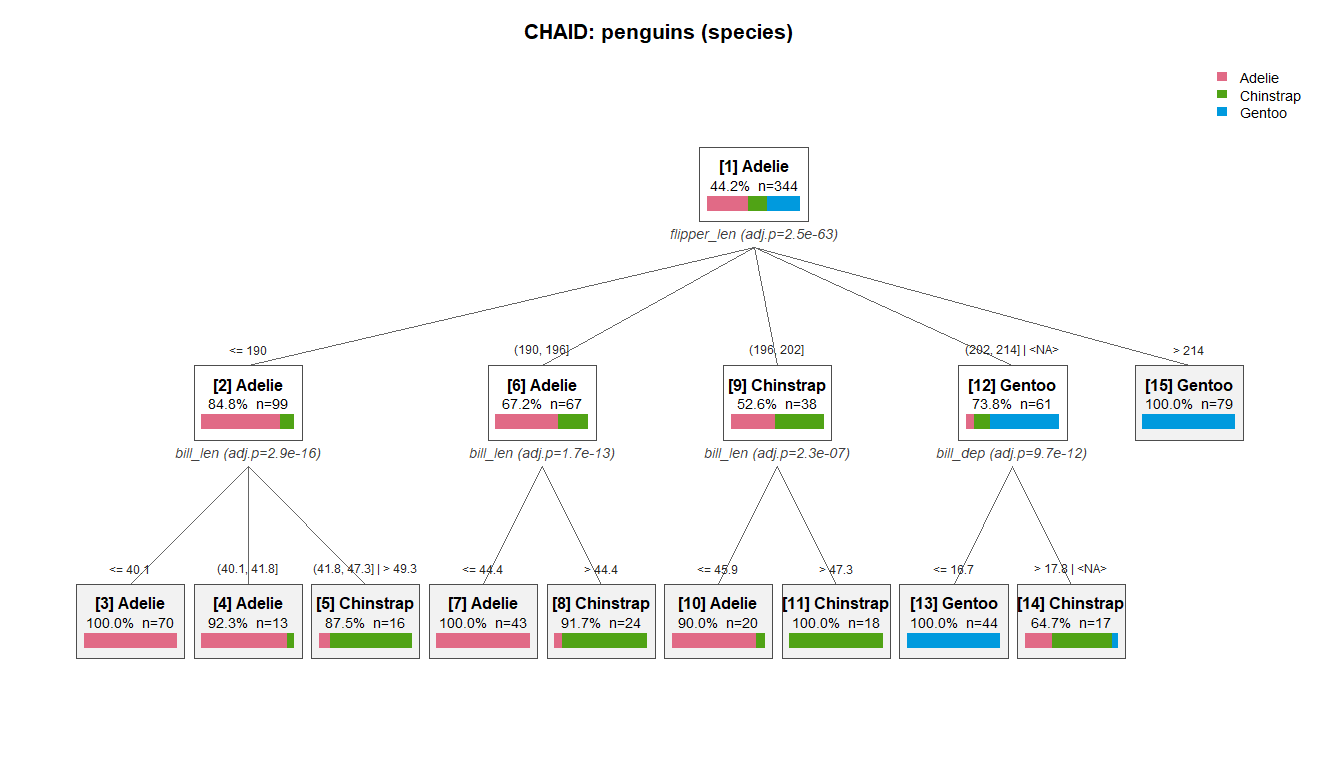

Prediction uses the standard S3 predict() interface:

pred <- predict(fit, penguins)          # class labels (factor)
mean(pred == penguins$species)          # training accuracy
#> [1] 0.9622093

round(predict(fit, head(penguins, 3), type = "prob"), 3)
#>      Adelie Chinstrap Gentoo
#> [1,]      1         0      0
#> [2,]      1         0      0
#> [3,]      1         0      0

Decision rules for every terminal node:

chaid_rules(fit)
#>    node
#> 1     3
#> 2     4
#> 3     5
#> 4     7
#> 5     8
#> 6    10
#> 7    11
#> 8    13
#> 9    14
#> 10   15
#>                                                                                                  rule
#> 1                                                             bill_len <= 40.1 and flipper_len <= 190
#> 2                                                     bill_len in (40.1, 41.8] and flipper_len <= 190
#> 3                                (bill_len in (41.8, 47.3] or bill_len > 49.3) and flipper_len <= 190
#> 4                                                      bill_len <= 44.4 and flipper_len in (190, 196]
#> 5                                                       bill_len > 44.4 and flipper_len in (190, 196]
#> 6                                                      bill_len <= 45.9 and flipper_len in (196, 202]
#> 7                                                       bill_len > 47.3 and flipper_len in (196, 202]
#> 8                          bill_dep <= 16.7 and (flipper_len in (202, 214] or flipper_len is missing)
#> 9  (bill_dep > 17.8 or bill_dep is missing) and (flipper_len in (202, 214] or flipper_len is missing)
#> 10                                                                                  flipper_len > 214

Key functions

Documentation

• vignette("chaidr") – a compact introduction (in English).
• vignette("chaidr-ja") – a detailed tutorial covering the algorithm, all option settings, evaluation, and visualization (in Japanese).

References

• Kass, G. V. (1980). An exploratory technique for investigating large quantities of categorical data. Applied Statistics, 29(2), 119–127.
• Biggs, D., de Ville, B., & Suen, E. (1991). A method of choosing multiway partitions for classification and decision trees. Journal of Applied Statistics, 18(1), 49–62.
• IBM Corp. IBM SPSS Statistics Algorithms – “CHAID and Exhaustive CHAID Algorithms”.

Acknowledgments

Development of this package was assisted by Google Gemini and Claude Code (Anthropic).

License

MIT (c) Osamu Morimoto