

fastgbm is a fast gradient boosting engine for R, with a
compiled (Rcpp + RcppParallel) backend, covering four task types with
one interface: regression (squared error), binary and multiclass
classification (logistic and one-vs-rest), and right-censored survival
analysis (Cox, AFT, or piecewise-exponential objectives). Survival is
where the package differentiates itself from general-purpose GBM
packages: xgboost has a Cox objective but no
baseline-hazard/survival-curve prediction built in, and general-purpose
GBM packages don’t route missingness natively for survival-specific
workflows. fastgbm gives you a single function call that
handles training, native missing-value routing, and (for survival
objectives) baseline hazard estimation and survival-probability
prediction at chosen horizons.
fastgbm()):
objective = "regression" - squared error;objective = "binary" - logistic classification (0/1
response or two-level factor);objective = "multiclass" - one-vs-rest binary
classification (a fastgbm sub-model per class, sharing the
same hyperparameters); predict(type = "prob") renormalizes
the K binary probabilities to sum to 1,
predict(type = "class") is their argmax;objective = "cox" / "aft" /
"pexp" - right-censored survival analysis. Cox uses Breslow
ties, AFT a normal location-scale error, and pexp
(piecewise-exponential) models the hazard jointly over covariates
and time via a person-time expansion (the standard Poisson
trick), rather than assuming a fixed post-hoc baseline like Cox’s
Breslow estimator - see
vignette("survival", package = "fastgbm").objective can be omitted: it is inferred from
y (a survival::Surv response or
time/status defaults to "cox"; a
0/1 or two-level-factor y defaults to
"binary"; a factor/character y with 3+ levels
defaults to "multiclass"; anything else numeric defaults to
"regression").y ~ . /
Surv(time, status) ~ .) interfaces;validation = list(x=, y=) for regression/binary, or
list(x=, time=, status=) for survival,
early_stopping = <patience>) - stops when the
held-out loss stops improving and keeps the best-iteration model; see
Scientific validity below for why this matters;threads = 0L for
automatic; identical fitted values regardless of thread count, including
with early stopping active);pdp()), and
serialization helpers, shared across all four task types.New objectives (each needs a derived
gradient/Hessian, a finite-difference validation pass, and a documented
estimand before any code is written, per this project’s own rule against
undocumented new losses): * A native K-tree softmax multiclass objective
(a single compiled kernel producing all K class scores per round) as an
alternative to the current one-vs-rest
objective = "multiclass" wrapper. * RMST-oriented loss -
undesigned. * Royston-Parmar-style flexible spline hazard-surface
objective - undesigned; harder than pexp because the
spline’s hazard derivative w.r.t. log-time would need finite differences
of the (non-differentiable) tree ensemble. * AFT distributions beyond
the normal (logistic, extreme value).
Engine / training * Leaf-wise
(grow_policy = "lossguide") tree growth - depth-wise only
currently. * Monotonic and interaction constraints. * Parallel
prediction - only the training split search is parallelized
(RcppParallel); prediction is single-threaded. * An \(O(n \log n)\) concordance implementation -
the internal C-index helper (fastgbm:::survival_cindex())
is still \(O(n^2)\), fine at the sample
sizes benchmarked so far but a real bottleneck for larger cohorts.
Explored, tested, but not adopted (results were
dataset-dependent, not a universal win - see
paper/fastgbm-benchmark.qmd Roadmap for the numbers): * An
mtry-scaled-to-sqrt(p)/p
colsample default (helped on higher-p
datasets, hurt on low-p ones). * A
bagged-ensemble-of-fastgbm-fits wrapper, bootstrap
resampling + averaging, directly borrowing ranger’s bagging
mechanism (closed the C-index gap to ranger on some
datasets, not others).
API-level * pexp’s
predict(type = "link"/"response") uses the cumulative
hazard at the model’s fitted time horizon as a risk score, since there’s
no single scalar “linear predictor” the way Cox/AFT have one - correct,
but coarser and slower to compute than the other two objectives. *
Cross-platform CI (GitHub Actions) now runs
R CMD check --as-cran on every push; win-builder/R-hub
checks are still pending before an actual CRAN submission, and the
GitHub repository is currently private (which will 404 CRAN’s URL check
until it’s made public).
Every objective’s gradient/Hessian has been checked against finite
differences of its stated loss, the Cox baseline-hazard estimator has
been checked against survival::basehaz(), missing-value and
numerical-edge-case behavior is stress-tested, and training is checked
to be bit-identical across thread counts (see
tests/testthat/test-gradients.R,
test-survival-validity.R, test-missing.R,
test-safeguards.R, test-parallel.R). This
audit found and fixed four real defects in the pre-rename implementation
(a sign error in the AFT censored-observation gradient/Hessian, a
Breslow baseline hazard whose risk set never shrank over time, a sign
error in the AFT concordance score, and a crash in
importance()) - see NEWS.md for details.
R CMD check is clean (0 errors, 0 warnings).
R CMD build .
R CMD INSTALL fastgbm_0.6.0.tar.gzlibrary(fastgbm)
# regression
fit_reg <- fastgbm(as.matrix(mtcars[, c("cyl", "disp", "hp", "wt")]), y = mtcars$mpg)
predict(fit_reg, mtcars[1:5, c("cyl", "disp", "hp", "wt")])
# binary classification
fit_bin <- fastgbm(as.matrix(mtcars[, c("mpg", "disp", "hp", "wt")]), y = mtcars$am, objective = "binary")
predict(fit_bin, mtcars[1:5, c("mpg", "disp", "hp", "wt")], type = "response") # probabilities
# multiclass classification (one-vs-rest)
fit_multi <- fastgbm(as.matrix(iris[, 1:4]), y = iris$Species)
predict(fit_multi, iris[1:5, 1:4], type = "prob") # per-class probabilities
predict(fit_multi, iris[1:5, 1:4], type = "class") # predicted class labels
# survival
library(survival)
lung_dat <- na.omit(lung[, c("time", "status", "age", "sex", "ph.ecog")])
fit_surv <- fastgbm(
as.matrix(lung_dat[, c("age", "sex", "ph.ecog")]),
time = lung_dat$time,
status = lung_dat$status,
objective = "cox"
)
predict(fit_surv, lung_dat[1:5, c("age", "sex", "ph.ecog")], type = "survival", times = c(90, 180, 365))
# formula interface works for all four:
fastgbm(mpg ~ cyl + disp + hp + wt, data = mtcars)
fastgbm(Surv(time, status) ~ age + sex + ph.ecog, data = lung_dat)See vignette("getting-started", package = "fastgbm"),
vignette("regression", package = "fastgbm"),
vignette("classification", package = "fastgbm"), and
vignette("survival", package = "fastgbm") for more.
A reproducible benchmark
(inst/benchmarks/run-benchmark.R) compares all three
fastgbm objectives (cox, aft,
pexp) against gbm, xgboost, and
ranger on 6 real survival datasets from the
biostatlab package.
gbm/xgboost/ranger use a fixed
ntrees = 200; each fastgbm arm uses
ntrees = 200 as a ceiling with validation-based early
stopping active (15% of its training fold held out, patience 20 rounds)
- error-analysis diagnostics
(inst/benchmarks/error-analysis/) showed test C-index
consistently peaked well before 200 rounds without it, and that
colsample/subsample resampled at every tree
node (like ranger’s mtry, not xgboost-style
per-tree sampling) further improves both speed and C-index. All arms
share max_depth = 5, learning_rate = 0.1,
min_node_size = 10, single-threaded, over 10 repeated 70/30
splits; fastgbm uses its
subsample = 0.8/colsample = 0.8 defaults.
Median training time and Harrell’s C-index (fastgbm’s
best-performing objective per dataset shown, all three reported in the
paper):
| dataset (n) | fastgbm (best objective) | gbm | xgboost | ranger |
|---|---|---|---|---|
| pbc (276) | 0.006s / 0.809 (cox) | 0.028s / 0.804 | 0.049s / 0.819 | 0.123s / 0.820 |
| heart_failure (299) | 0.003s / 0.706 (cox) | 0.019s / 0.681 | 0.028s / 0.682 | 0.072s / 0.728 |
| breast (672) | 0.006s / 0.666 (aft) | 0.031s / 0.648 | 0.038s / 0.648 | 0.222s / 0.697 |
| colon_cancer (888) | 0.155s / 0.629 (pexp) | 0.047s / 0.645 | 0.035s / 0.609 | 0.193s / 0.655 |
| crc_mondaca2020 (471, real missingness) | 0.005s / 0.576 (cox) | 0.038s / 0.558 | 0.042s / 0.553 | 0.148s / 0.612 |
| framingham (5209) | 0.053s / 0.757 (cox, beats ranger’s 0.756 on median) | 0.267s / 0.759 | 0.080s / 0.747 | 2.396s / 0.756 |
(bold = fastgbm beats both gbm and xgboost on median C-index)
(training seconds / Harrell’s C-index, both medians across 10 repeated 70/30 splits)
Honest summary, not a universal-superiority claim:
fastgbm’s cox arm is now 5-9x faster to train
than gbm/xgboost and 22-45x faster than
ranger on every dataset, and beats both gbm
and xgboost on median C-index on 4-5 of 6 datasets
depending on objective. ranger’s discrimination lead
narrowed substantially (e.g. breast: gap went from 5.9
points of C-index to 2.0) and, on framingham,
cox’s median C-index now edges past ranger’s
(0.757 vs. 0.756) - though not consistently enough across repeated
splits to count as a clear win in the paired comparison, and
ranger remains ahead on the other five datasets.
pexp is markedly slower than
cox/aft (it evaluates the ensemble once per
time interval, not once per row) and is currently the strongest
objective on only one dataset (colon_cancer). See
paper/fastgbm-benchmark.qmd (renders to
fastgbm-benchmark.pdf) for the full write-up with
repeated-split uncertainty, paired win/loss/tie counts, and the
threads=1-vs-N parallelism results;
inst/benchmarks/benchmark-results.csv /
benchmark-summary.csv / parallel-speedup.csv
for the raw and aggregated numbers; and
inst/benchmarks/session-info.txt for reproducibility
metadata.
The earlier single-dataset survival::lung benchmark is
still available via tools/benchmark-survival.R /
inst/benchmarks/survival-cox-lung.csv.
A second reproducible benchmark
(inst/benchmarks/run-benchmark-regression.R) checks the
"regression" objective on Friedman’s #1 DGP
(mlbench::mlbench.friedman1()), the standard synthetic
nonlinear-regression benchmark used in the gradient boosting
literature:
y = 10*sin(pi*x1*x2) + 20*(x3 - 0.5)^2 + 10*x4 + 5*x5 + epswith x1-x10 iid Uniform(0, 1) and only
x1-x5 entering the mean function
(x6-x10 are pure noise). This DGP is useful
precisely because the true functional form is known, so both predictive
accuracy and whether the model recovers the right shape per
feature can be checked, not just average error. Same regime as the
survival benchmark: fastgbm
vs. gbm/xgboost/ranger, equal
ntrees = 200 (ceiling for fastgbm, which uses
early stopping)/
max_depth = 5/learning_rate = 0.1/min_node_size = 10,
single-threaded, 10 repeated 70/30 splits on n = 2000.
Computational time and accuracy (training seconds / test-set RMSE, both medians across repeats):
| model | train time | RMSE |
|---|---|---|
| fastgbm | 0.087s | 1.386 |
| gbm | 0.143s | 1.281 |
| xgboost | 0.198s | 1.388 |
| ranger | 0.102s | 2.594 |
fastgbm trains ~1.6-2.3x faster than
gbm/xgboost (win/loss/tie 10/0/0 vs. each,
paired across repeats) and now beats ranger on
median training time (win/loss/tie 7/3/0, fastgbm’s own
median: 0.087s vs. ranger’s 0.102s), while clearly beating
ranger on RMSE (10/0/0) and roughly matching
xgboost (6/4/0); gbm edges out
fastgbm on RMSE here (0/10/0). Consistent with the survival
benchmark: fastgbm is not a universal-accuracy win, but it
is never far off and is now the fastest of the four on this benchmark,
not just competitive – see “Split-search optimizations” and “Level-wise
tree growth” below for what closed (and then reversed) the gap to
ranger.
For a closer look at the distribution of training time, not
just the median, inst/benchmarks/run-benchmark-exectime.R
times all four models (explicitly checked to grow the same
ntrees = 200 each, so the comparison is purely about
training-algorithm speed) on one fixed 2,000-row Friedman1 draw with bench::mark()
(benchr, originally used for this, was archived off CRAN in
November 2025; bench is the actively maintained
equivalent), which reruns each model until it has collected at least 10
timings:
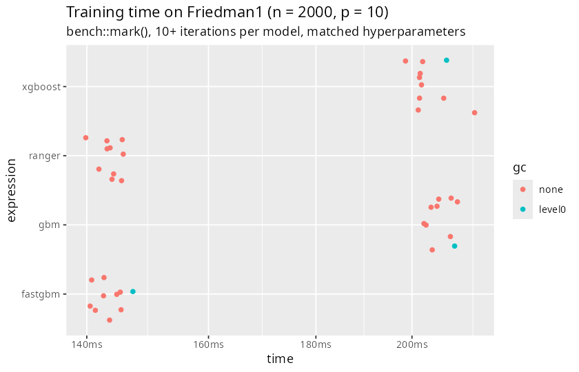
fastgbm and ranger overlap almost entirely
around 141-150ms, both clearly separated from
gbm/xgboost’s 199-234ms band. See
inst/benchmarks/regression-exectime-bench.csv for the full
bench::mark() summary
(min/median/itr/sec/memory allocation).
Three changes to src/fastgbm.cpp’s split search closed,
then reversed, the gap to ranger shown above
(fastgbm went from training 1.3-1.8x faster than
gbm/xgboost but noticeably behind
ranger, to now beating all three; see NEWS.md
for the exact before/after numbers at each step):
RcppParallel::parallelFor() was still being dispatched
for large-enough nodes even when threads = 1L was
requested, paying real thread-pool scheduling overhead for work that
only ever ran on one thread. A single explicit thread request now always
takes the direct (serial) call path, regardless of node/feature
size.G/H, needed both for the leaf value and the
split-gain formula) with a fresh full pass over its rows – but those
exact sums were already produced as a byproduct of the parent’s
winning split
(GL/HL/GR/HR in the
histogram scan above). Passing them down instead of recomputing removes
a second full pass per node, on top of the split search itself.The first two changes are exactly behavior-preserving (bit-identical
split decisions and benchmark output). The third is not – it sums the
same grad/Hessian values in a different order (histogram-bin order for a
child’s inherited G/H, vs. row order for a
fresh sum), which is a legitimate floating-point reassociation, not a
bug, but can occasionally tip a near-tied split threshold and lead to a
different-but-equally-valid tree. This was verified directly, not just
assumed: a dedicated test
(tests/testthat/test-tree-building.R) independently
recomputes each leaf’s -G/(H+lambda) in R from the actual
rows that reach it (with subsample/ colsample
fixed at 1 so the true set of rows is unambiguous) and
checks it against the compiled value to 1e-10 – along with
the full existing test suite (thread-count-determinism,
finite-difference gradient/Hessian checks), all passing.
The single n = 2000/p = 10 snapshot above
is not the whole story: ranger parallelizes across
trees (embarrassingly parallel, since random-forest trees are
independent), while fastgbm’s boosting is sequential across
trees and only parallelizes within a tree’s split search – so
how the two compare depends on data shape and thread count, not just one
point. inst/benchmarks/run-benchmark-scaling.R sweeps
n in {1000, 5000, 20000} and p in
{10, 50, 100, 1000} (Friedman1’s 10 columns plus pure-noise
columns to reach the target p), single-threaded, 100 trees,
matched hyperparameters:

Two clear patterns: fastgbm’s relative speed improves as
n grows (fastgbm/ranger training-time ratio goes
from 1.20x at n=1000, p=10 to 0.52x at
n=20000, p=10 – crossing over from slower to faster), but
degrades as p grows (1.20x -> 3.15x
-> 4.45x -> 12.04x at n=1000 as p goes
10 -> 50 -> 100 -> 1000). The p effect traces to a
real, fixable cause, not an engine inefficiency: fastgbm’s
default colsample = 0.8 searches ~80% of features at every
split regardless of p, while ranger’s default
mtry for regression is p/3 – at
p = 1000 that is 800 features searched per split vs. 333.
Setting fastgbm’s colsample to match
(1/3 here) confirms it: at n = 5000, p = 100,
training time drops from 0.98s (colsample = 0.8) to 0.50s
(colsample = 1/3), turning a loss to ranger
(0.57s) into a win. The trade-off is real too –
colsample = 0.8 was the package’s own tuned default for a
reason (see ?fastgbm: it gave a small but consistently
non-negative C-index gain on the survival benchmark datasets), so this
is a speed/accuracy dial, not a free lunch. Note that n
growing does not always rescue fastgbm from a
high-p disadvantage the way it does at
p <= 100: at p = 1000, fastgbm
is still ~2.8x slower than ranger even at the largest
n tested (n = 20000), the one p
in this grid where growing n alone was not enough to close
the gap – colsample tuning matters most exactly here.
The thread sweep
(inst/benchmarks/run-benchmark-scaling.R, at the largest
grid point, n = 20000, p = 1000, on a 16-core machine)
shows real but sub-linear speedup, as expected for within-tree (not
across-tree) parallelism – and better scaling than the smaller
p = 100 grid point used in earlier versions of this
section, since a wider colsample-sampled feature set gives
the level-wise split search more to parallelize per level:
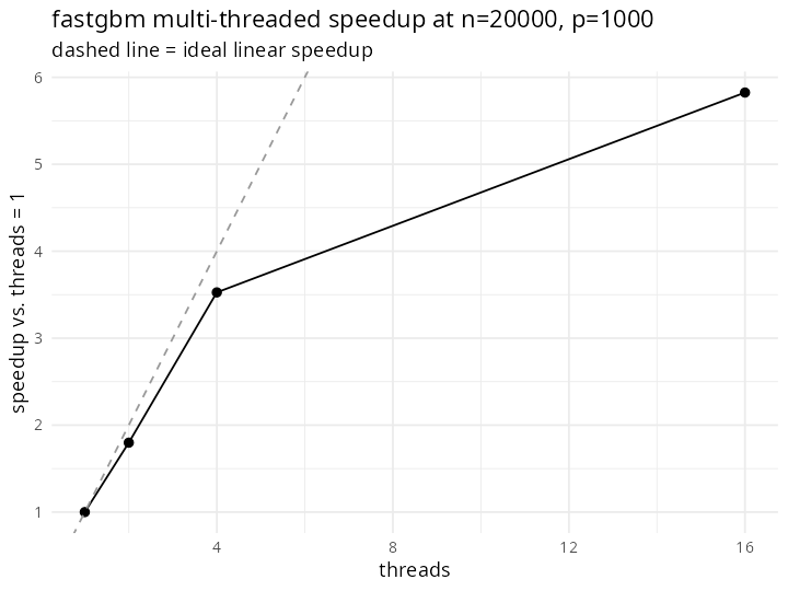
1.8x at 2 threads, 3.5x at 4 threads, 5.8x at 16 threads (with the
level-wise tree-growth engine described further below; the same sweep at
p = 100 reached only ~3.0x at 16 threads) – real, and
clearly improved at high p, but still nowhere near the
dashed ideal-linear line, and not worth reaching for on small data
(threads = 1L already skips parallelFor()’s
dispatch overhead entirely; see “Split-search optimizations” above).
Everything above (including “fastgbm now beats
ranger” earlier in this section) was single-threaded.
ranger and xgboost also support
multi-threading, and each parallelizes completely differently from
fastgbm: ranger splits independent
trees across threads (embarrassingly parallel),
xgboost’s histogram build is parallelized more thoroughly
across both rows and features, and fastgbm (see “Level-wise
tree growth” below) parallelizes the combined split-search workload
across every node active at one tree level at a time.
inst/benchmarks/run-benchmark-multithreaded.R checks this
directly at n = 20000, p = 100 (the largest grid point
above), threads in {1, 4, 12}, median of 5 repeats
(gbm has no thread-count control for a single fit and is
shown only as a fixed single-threaded reference line):
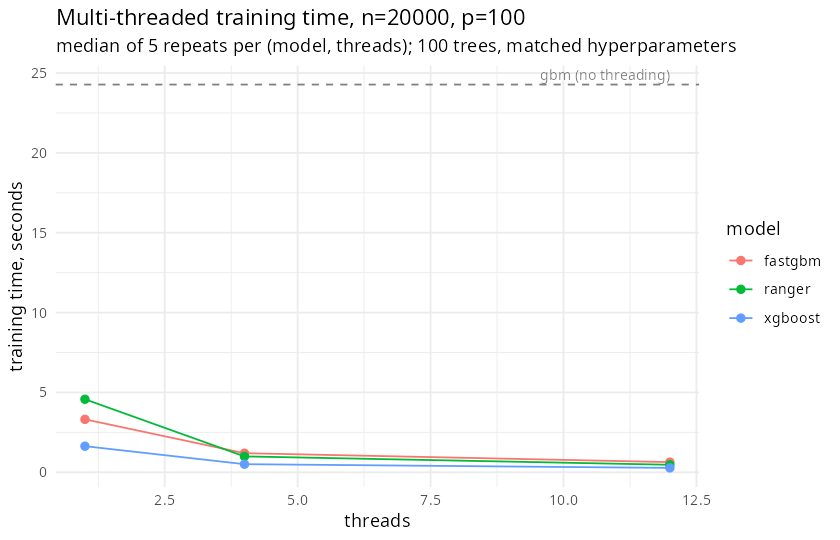
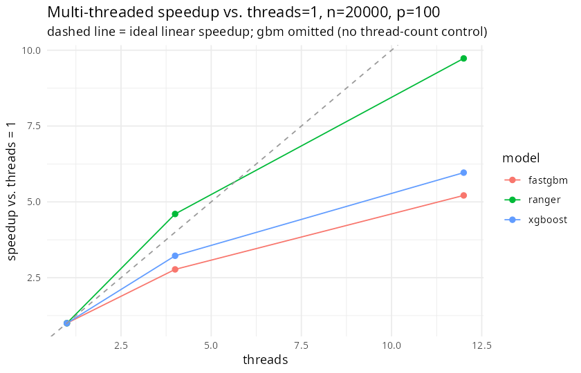
At threads = 1, fastgbm (~3.3s) is faster
than ranger (~4.6s), matching the single-threaded story
above, though both are behind xgboost (~1.6s) at this large
n x p (absolute times here run a bit higher across all
models than the scaling-sweep numbers above – machine load varies
between runs; what is stable across repeated runs of this benchmark is
the relative ordering and shape of the three speedup curves,
which is what matters for the conclusion below). By
threads = 12, fastgbm reaches ~5.2x speedup
vs. ranger’s ~9.7x and xgboost’s ~6.0x – so in
absolute terms fastgbm (~0.64s) ends up the
slowest of the three at this thread count, behind
ranger (~0.47s) and xgboost (~0.27s). The
takeaway is not “fastgbm is slow” – it is that
fastgbm’s speed advantage is concentrated in the
single-/few-threaded regime, because its parallelism has
structurally less to work with per dispatch than an entire forest’s
independent trees or a histogram build parallelized across rows and
features both. If your workflow already runs on a many-core machine and
wall-clock time is the only thing that matters,
ranger/xgboost at a high thread count may
still win even where fastgbm wins single-threaded.
An earlier version of src/fastgbm.cpp parallelized the
split search once per node (across that node’s own sampled features).
That works fine near the root, but a single node’s row/feature count
shrinks fast with depth, while the fixed cost of dispatching a
parallelFor() call does not – so by a few levels in, most
nodes no longer had enough work to make parallel dispatch worthwhile,
and multi-threading’s benefit tailed off deep in the tree, right where a
lot of the total node count actually lives.
build_tree() now grows a tree breadth-first, one full
level at a time: every node active at the current depth has its
split-search tasks (one per sampled feature) pooled into a single
combined batch before any of them run, and that whole batch is what
gets parallelized. This keeps the per-dispatch work large even deep in a
tree, because each level roughly doubles its node count while roughly
halving each node’s row count – the total combined work per level stays
close to constant, unlike a single node’s shrinking share of it.
Verified two ways before trusting it: the existing leaf-value
correctness test (independently recomputing -G/(H+lambda)
from the actual rows reaching each leaf) and a new
multi-threaded-vs-single-threaded identical-tree check both pass
(tests/testthat/test-tree-building.R), confirming the new
growth order is still exactly correct and still
thread-count-deterministic, even though tree structure differs from the
earlier depth-first version (it draws colsample subsets in
a different, but equally valid, order).
Net effect, same n = 20000, p = 100 setup as the
head-to-head above: fastgbm’s own speedup improved from
1.9x/3.3x (4/12 threads, prior per-node dispatch) to
2.8x/5.2x – a real, measured gain, not just a
plausible-sounding idea (a first attempt, increasing
parallelFor()’s grain size to reduce per-task scheduling
overhead, was tried and measured worse, and was reverted – see
NEWS.md). It narrows the gap to
ranger/xgboost’s steeper scaling curves
without closing it; matching a fully independent per-tree or
per-row-block parallelism model would need a larger, different change
than tuning the existing within-level split search further.
Tuning tips for runtime, in rough order of expected impact:
p: lower colsample.
The single biggest lever found here. Try something in
ranger’s ballpark (~1/3, or
sqrt(p)/p for very wide data) and check whether the
accuracy cost is acceptable for your dataset – it was small-to-neutral
on every survival benchmark dataset tested so far, but that is not a
guarantee for every dataset.ranger/xgboost at a high thread count too
before assuming fastgbm wins.
fastgbm’s own threads (explicit, or
0L for automatic) still helps in absolute terms –
parallelism pays off once a tree level’s combined task count crosses the
internal parallelFor() threshold (>= 8 tasks) – but its
speedup curve is flatter than either competitor’s even after the
level-wise rewrite above (see the head-to-head), so it is not guaranteed
to still be the fastest option once every candidate is allowed to use
all available cores.n: don’t expect threading or
colsample to matter much. At
n = 1000, fixed per-tree overhead (R/C++ call marshaling,
tree-object allocation) is a larger share of total time, so the sweep
above shows fastgbm closest to (or behind)
ranger exactly in this regime, regardless of these
settings.subsample < 1) reduces the
rows scanned in every split search roughly linearly – an
orthogonal lever to colsample, stackable with it, at a
similar speed/accuracy trade-off (the package default is
0.8, already below 1).max_depth and
min_node_size trade tree count for training time roughly
like colsample trades feature count for it, just via a
different axis (fewer nodes visited vs. less searched per node).See
inst/benchmarks/scaling-benchmark-np.csv/scaling-benchmark-threads.csv
for the full numbers behind the n/p/single-model-thread plots, and
inst/benchmarks/multithread-benchmark.csv for the
multi-threaded head-to-head.
PDP shape recovery: since the true partial
dependence of each feature is computable in closed form for this DGP
(fixing x_j on a grid and averaging the true mean function
over the observed rows), pdp() on the fitted
fastgbm model can be checked directly against ground truth
rather than just inspected by eye:

fastgbm’s partial dependence tracks the true shape
closely for all four plotted features: the x1*x2
interaction correctly flattens x1’s marginal effect into a
shallow hump (not the raw sin curve, since x2
is averaged out), x3’s quadratic term is recovered as a
clean U-shape, and x4/x5’s linear terms are
recovered as straight lines. See
inst/benchmarks/regression-pdp-data.csv for the underlying
numbers and inst/benchmarks/regression-session-info.txt for
reproducibility metadata.