![]()

The main aim of the gamlssx package is to enable a
generalized extreme value (GEV) to be used as the response distribution
in a generalized additive model for location scale and shape (GAMLSS),
as implemented in the gamlss R package.
The gamlss.dist R
package does offer reversed GEV distribution via in RGE
family, but (a) this is not the usual parameterization of a GEV
distribution (for block maxima), and (b) in RGE, the shape
parameter is restricted to have a particular sign, which is undesirable
because the sign of the shape parameter influences strongly extremal
behaviour. The gamlssx package uses the usual
parameterization, with a shape parameter \(\xi\), and imposes only the restriction
that, for each observation in the data, \(\xi
> -1/2\), which is necessary for the usual asymptotic
likelihood theory to be applicable.
See Rigby and Stasinopoulos (2005) and the gamlss home page for details of the GAMLSS methodology. See also Gavin Simpson’s blog post Modelling extremes using generalized additive models for an overview of the use of GAMs for modelling extreme values, which uses the mgcv R package to fit similar models. The VGAM and evgam R packages can also be used.
We consider the fremantle data include in the
gamlssx package, which is a copy of data of the same name
from the ismev R
package. These data contain 86 annual maximum seas levels recorded
at Fremantle, Australia during 1987-1989. In addition to the year of
each sea level, we have available the value of the Southern Oscillation
Index (SOI). We use the fitGEV() function provided in
gamlssx to fit a model to these data that is similar to the
first one fitted, to the same data, in Gavin Simpson’s blog post.
The fitGEV() function calls the function
gamlss::gamlss(), which offers 3 fitting algorithms:
RS (Rigby and Stasinopoulos), CG (Cole and
Green) and mixed (RS initially followed by
CG). In the code below, we use the default RS
algorithm. fitGEV() offers 2 scoring methods to calculate
the weights used in the algorithm. Here, we use the default, Fisher’s
scoring, based on the expected Fisher information. The code below does
not do justice to the functionality of the gamlss package.
See the GAMLSS
books for more information.
# Load gamlss, for the function term.plot()
library(gamlss)
# Load gamlssx
library(gamlssx)
# Transform Year so that it is centred on 0
fremantle <- transform(fremantle, cYear = Year - median(Year))
# Plot sea level against year and against SOI
plot(fremantle$Year, fremantle$SeaLevel, xlab = "year", ylab = "sea level (m)")
plot(fremantle$SOI, fremantle$SeaLevel, xlab = "SOI", ylab = "sea level (m)")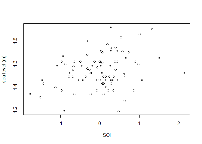
# Fit a model with P-spline effects of cYear and SOI on location and scale
# The default links are identity for location and log for scale
mod <- fitGEV(SeaLevel ~ pb(cYear) + pb(SOI),
              sigma.formula = ~ pb(cYear) + pb(SOI),
              data = fremantle)
#> GAMLSS-RS iteration 1: Global Deviance = -112.2422
#> GAMLSS-RS iteration 2: Global Deviance = -117.4965
#> GAMLSS-RS iteration 3: Global Deviance = -118.3007
#> GAMLSS-RS iteration 4: Global Deviance = -118.6081
#> GAMLSS-RS iteration 5: Global Deviance = -118.7582
#> GAMLSS-RS iteration 6: Global Deviance = -118.8344
#> GAMLSS-RS iteration 7: Global Deviance = -118.8731
#> GAMLSS-RS iteration 8: Global Deviance = -118.8987
#> GAMLSS-RS iteration 9: Global Deviance = -118.9102
#> GAMLSS-RS iteration 10: Global Deviance = -118.9188
#> GAMLSS-RS iteration 11: Global Deviance = -118.9258
#> GAMLSS-RS iteration 12: Global Deviance = -118.9269
#> GAMLSS-RS iteration 13: Global Deviance = -118.9351
#> GAMLSS-RS iteration 14: Global Deviance = -118.9359
# Summary of model fit
summary(mod)
#> ******************************************************************
#> Family:  c("GEV", "Generalized Extreme Value")
#>
#> Call:  gamlss::gamlss(formula = SeaLevel ~ pb(cYear) + pb(SOI),
#>     sigma.formula = ~pb(cYear) + pb(SOI), family = GEVfisher(mu.link = "identity",
#>         sigma.link = "log", nu.link = "identity"),
#>     data = fremantle, mu.step = c(1, 1, 1)[1], sigma.step = c(1,
#>     1, 1)[2], nu.step = c(1, 1, 1)[3])
#>
#> Fitting method: RS()
#>
#> ------------------------------------------------------------------
#> Mu link function:  identity
#> Mu Coefficients:
#>              Estimate Std. Error t value Pr(>|t|)
#> (Intercept) 1.5007933  0.0149733 100.231  < 2e-16 ***
#> pb(cYear)   0.0019490  0.0004982   3.912 0.000195 ***
#> pb(SOI)     0.0680347  0.0174751   3.893 0.000208 ***
#> ---
#> Signif. codes:  0 '***' 0.001 '**' 0.01 '*' 0.05 '.' 0.1 ' ' 1
#>
#> ------------------------------------------------------------------
#> Sigma link function:  log
#> Sigma Coefficients:
#>              Estimate Std. Error t value Pr(>|t|)
#> (Intercept) -2.128696   0.088447 -24.068   <2e-16 ***
#> pb(cYear)   -0.004574   0.002614  -1.750   0.0841 .
#> pb(SOI)      0.275258   0.112736   2.442   0.0169 *
#> ---
#> Signif. codes:  0 '***' 0.001 '**' 0.01 '*' 0.05 '.' 0.1 ' ' 1
#>
#> ------------------------------------------------------------------
#> Nu link function:  identity
#> Nu Coefficients:
#>             Estimate Std. Error t value Pr(>|t|)
#> (Intercept) -0.25619    0.08582  -2.985  0.00379 **
#> ---
#> Signif. codes:  0 '***' 0.001 '**' 0.01 '*' 0.05 '.' 0.1 ' ' 1
#>
#> ------------------------------------------------------------------
#> NOTE: Additive smoothing terms exist in the formulas:
#>  i) Std. Error for smoothers are for the linear effect only.
#> ii) Std. Error for the linear terms maybe are not accurate.
#> ------------------------------------------------------------------
#> No. of observations in the fit:  86
#> Degrees of Freedom for the fit:  8.375675
#>       Residual Deg. of Freedom:  77.62432
#>                       at cycle:  14
#>
#> Global Deviance:     -118.9359
#>             AIC:     -102.1846
#>             SBC:     -81.62773
#> ******************************************************************
# Model diagnostic plots
plot(mod)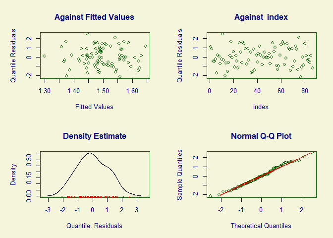
#> ******************************************************************
#>        Summary of the Quantile Residuals
#>                            mean   =  -0.006109438
#>                        variance   =  1.036755
#>                coef. of skewness  =  0.09394729
#>                coef. of kurtosis  =  2.322565
#> Filliben correlation coefficient  =  0.9951795
#> ******************************************************************
# Plot of the fitted component smooth functions
# Note: gamlss::term.plot() does not include uncertainty about the intercept
# Location mu
term.plot(mod, rug = TRUE, pages = 1)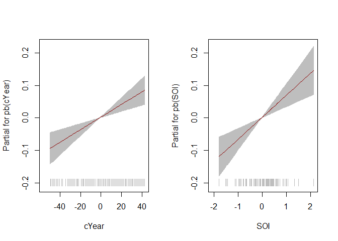
# Scale sigma
term.plot(mod, what = "sigma", rug = TRUE, pages = 1)
To get the current released version from CRAN:
install.packages("gamlssx")