



The R package icomb provides tools for implementing the information combination approach to forecasting hierarchical time series proposed by Nguyen, Vahid and Wickramasuriya (2025).
It offers tools to construct and combine forecasts based on different information sets, enabling improved forecast accuracy within hierarchical and grouped time series structures.
You can install the stable version on CRAN:
install.packages("icomb")You can install the development version from GitHub
# install.packages("pak")
pak::pak("ShanikaLW/icomb")library(fable)
library(fabletools)
library(tsibble)
library(dplyr)
library(lubridate)
library(icomb)
library(ggtime)
tourism_hts <- tourism |>
aggregate_key(State * Purpose,
Trips = sum(Trips))
fit <- tourism_hts |>
model(base = ETS(Trips)) |>
reconcile(ols = min_trace(base, method = "ols"),
icomb = icomb(base, train_size = 75))
fit
#> # A mable: 45 x 5
#> # Key: State, Purpose [45]
#> State Purpose base ols icomb
#> <chr*> <chr*> <model> <model> <model>
#> 1 ACT Business <ETS(M,N,M)> <ETS(M,N,M)> <ETS(M,N,M)>
#> 2 ACT Holiday <ETS(M,N,A)> <ETS(M,N,A)> <ETS(M,N,A)>
#> 3 ACT Other <ETS(M,N,N)> <ETS(M,N,N)> <ETS(M,N,N)>
#> 4 ACT Visiting <ETS(M,N,N)> <ETS(M,N,N)> <ETS(M,N,N)>
#> 5 ACT <aggregated> <ETS(M,A,N)> <ETS(M,A,N)> <ETS(M,A,N)>
#> 6 New South Wales Business <ETS(M,N,A)> <ETS(M,N,A)> <ETS(M,N,A)>
#> 7 New South Wales Holiday <ETS(M,N,A)> <ETS(M,N,A)> <ETS(M,N,A)>
#> 8 New South Wales Other <ETS(A,N,N)> <ETS(A,N,N)> <ETS(A,N,N)>
#> 9 New South Wales Visiting <ETS(A,N,A)> <ETS(A,N,A)> <ETS(A,N,A)>
#> 10 New South Wales <aggregated> <ETS(A,N,A)> <ETS(A,N,A)> <ETS(A,N,A)>
#> # ℹ 35 more rows
fit |>
forecast(h = "3 years") |>
filter(Purpose == "Holiday", State == "Victoria") |>
autoplot(filter(tourism_hts, Purpose == "Holiday",
State == "Victoria", year(Quarter) > 2010), level = NULL)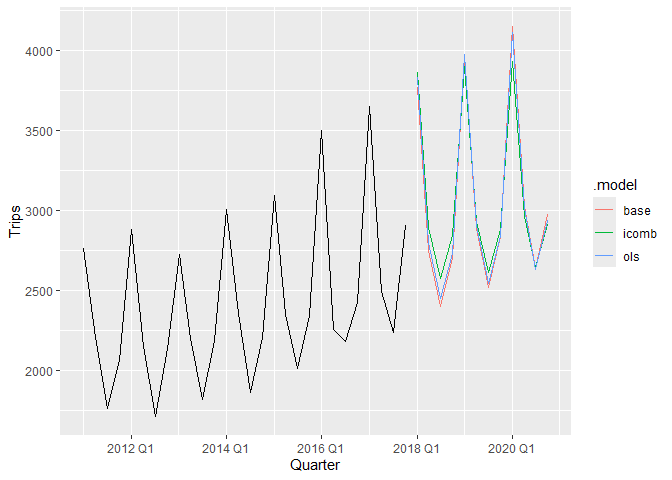 We
can compute probabilistic forecasts
We
can compute probabilistic forecasts
fit |>
  forecast(h = "3 years", bootstrap = TRUE, times = 1000) |>
  filter(Purpose == "Holiday", State == "Victoria") |>
  autoplot(filter(tourism_hts, Purpose == "Holiday",
                  State == "Victoria", year(Quarter) > 2010))
This workflow can be parallelized to improve performance using the
future package. By specifying a parallelization plan via
future::plan() (e.g., multisession or
multicore), users can control how computations are
distributed across available workers. This allows the cross-validation
procedure in the information combination approach to run in parallel
without modifying the core code, while remaining flexible to different
computing environments. If no plan is set, the default sequential
strategy is used, meaning computations are performed one after another
with no parallelization.
library(future)
plan(multisession, workers = 2)

tourism_hts |>
  model(base = ETS(Trips)) |>
  reconcile(ols = min_trace(base, method = "ols"),
            icomb = icomb(base, train_size = 75))  |>
  forecast(h = "3 years")
#> # A fable: 1,620 x 6 [1Q]
#> # Key:     State, Purpose, .model [135]
#>    State  Purpose  .model Quarter
#>    <chr*> <chr*>   <chr>    <qtr>
#>  1 ACT    Business base   2018 Q1
#>  2 ACT    Business base   2018 Q2
#>  3 ACT    Business base   2018 Q3
#>  4 ACT    Business base   2018 Q4
#>  5 ACT    Business base   2019 Q1
#>  6 ACT    Business base   2019 Q2
#>  7 ACT    Business base   2019 Q3
#>  8 ACT    Business base   2019 Q4
#>  9 ACT    Business base   2020 Q1
#> 10 ACT    Business base   2020 Q2
#> # ℹ 1,610 more rows
#> # ℹ 2 more variables: Trips <dist>, .mean <dbl>
plan(sequential)