BATTS implements the boosting and Bayesian additive tree methods from Awaya, Xu, and Ma (2025) for two-sample comparison through density ratio estimation.
Paper: Two-sample comparison through additive tree models for density ratios
library(devtools)
install_github("nawaya040/BATTS@v0.3.0")The official distribution is nawaya040/BATTS. From
version 0.3.0, the defaults of boots() and
batts() are the settings used in the paper’s simulations:
gradient boosting with at most 1000 trees selected by 5-fold CV, depth
4, learning rate 0.01 and per-tree subsampling of one half; and 200
Bayesian trees with 2000 burn-in iterations and 1000 saved draws. Calls
that relied on earlier defaults give different results; see NEWS.md. The paper’s simulations used version 0.2.2
(tag v0.2.2) with all settings supplied explicitly.
Versions 0.2.2 and 0.3.0 implement the same algorithms: 0.3.0 changes
only default argument values, and a fit with the same explicit arguments
and seed gives identical results in both versions.
For paper reproduction, use the exact BATTS commit recorded in the chosen simulation repository checkout. From that checkout’s root, the supported environment bootstrap is:
Rscript scripts/prepare_environment.R --install=true --r-lib=.RlibFor a package-only installation using the same pin, run from that simulation checkout’s root in a fresh R session:
source("config/study.R")
batts_sha <- study_config("smoke")$batts_sha
stopifnot(grepl("^[0-9a-f]{40}$", batts_sha))
remotes::install_github(paste0("nawaya040/BATTS@", batts_sha), upgrade = "never")
The smoke and paper profiles use the same dependency commit. Record
the simulation commit as well; selecting a moving branch does not freeze
it. Building from source requires a C++17 toolchain (Rtools on Windows).
Version 0.2.0 removed update_lambda,
lambda_prior_parameters, and alpha_cutpoint;
remove these named arguments from older calls. See NEWS.md for numerical changes in earlier versions.
Package commit, dependency versions, settings and seeds should accompany
each run.
This repository contains the estimator package, documentation, small examples and regression tests. Paper-scale simulations, comparator configurations, case-study data and reproduction workflows are maintained separately. The worked example below is an API demonstration with its own settings. It does not reproduce a specific paper table or establish MCMC convergence.
The example uses a shorter MCMC run than the defaults (2000 burn-in
iterations and 1000 draws) to finish quickly. Use
output_BART_ensembles = TRUE when posterior prediction at
new points is needed. Prediction outside the fitted domain is rejected.
All returned weights are sqrt(p/q); use
2 * log(w) for the full log-density ratio. Check mixing
across chains and sensitivity to limited overlap before interpreting
posterior intervals. Nominal pointwise intervals do not provide a
guarantee of frequentist coverage or simultaneous inference.
From version 0.4.0 the main user-facing functions are:
batts_boost() fits the boosting estimator, with
settings collected in boost_control().batts_bart() fits the Bayesian additive tree model,
with settings in bart_control(), and returns posterior
draws for uncertainty quantification.predict(), fitted() and
density_ratio() evaluate a fit; print(),
summary() and plot() describe it.The fitting functions accept a matrix, a data frame or a vector,
group labels of any two-valued type, or two samples
(batts_boost(x, y = y)).
boots(), batts() and
eval_balance_weight(), the interface of versions 0.1.0 to
0.3.0, still work and give the same results, but are deprecated. They
return the square root of the density ratio, so the worked example
below, written for that interface, converts outputs to log-density
ratios for plotting and interpretation.
The full example script is included in example.R.
The code below reproduces the main workflow.
library(mvtnorm)
library(ggplot2)
library(BATTS)

balance_to_log_ratio = function(x) {
  log(x) * 2
}

calc_quantiles = function(x) {
  quantile(x, probs = c(0.025, 0.975))
}set.seed(1)
n0 = 1000
n1 = 1000
X0 = rmvnorm(n0, mean = c(-0.5, -0.5))
X1 = rmvnorm(n1, mean = c(0.5, 0.5))
data = rbind(X0, X1)
group_labels = c(rep(0, n0), rep(1, n1))result_boosting = boots(
data = data,
group_labels = group_labels,
num_trees_max = 1000,
K_CV = 5,
max_resol = 4,
learn_rate = 0.01,
n_bins = 32,
margin_scale = 0.1,
use_gradient = TRUE,
subsample_fraction = 0.5,
quiet = TRUE
)
log_ratio_boosting =
balance_to_log_ratio(result_boosting$balance_weight_boosting_data)result_BAT = batts(
data = data,
group_labels = group_labels,
num_trees = 200,
lambda_0 = 5,
margin_scale = 0.1,
size_burnin = 500, # default 2000; shortened for the demonstration
size_backfitting = 500, # default 1000
output_BART_ensembles = TRUE,
quiet = TRUE
)
log_ratio_BAT = balance_to_log_ratio(result_BAT$balance_weight_BART_data)
log_ratio_BAT_mean = rowMeans(log_ratio_BAT)
log_ratio_BAT_quantiles = apply(log_ratio_BAT, 1, calc_quantiles)methods = c("GB", "BAT", "lower", "upper")
ratio_df = data.frame(
x = rep(data[, 1], 4),
y = rep(data[, 2], 4),
log_ratio = c(
log_ratio_boosting,
log_ratio_BAT_mean,
log_ratio_BAT_quantiles[1, ],
log_ratio_BAT_quantiles[2, ]
),
method = factor(rep(methods, each = nrow(data)), levels = methods)
)
max_abs = max(abs(ratio_df$log_ratio))
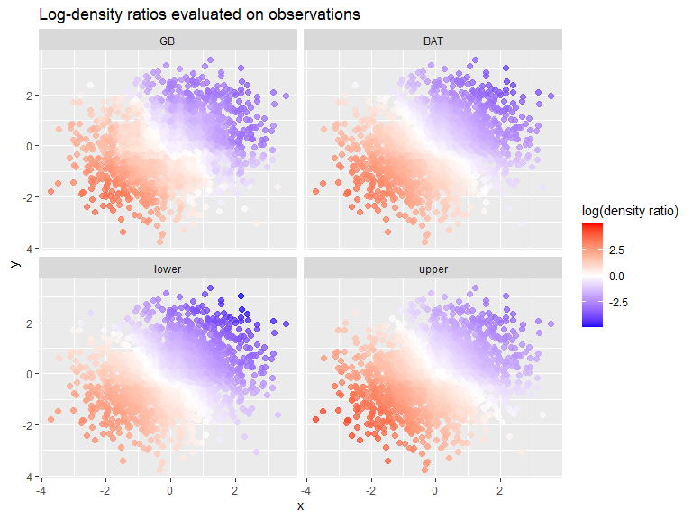
ggplot(ratio_df, aes(x = x, y = y, color = log_ratio)) +
geom_point(size = 2, alpha = 0.75) +
scale_color_gradientn(
colours = c("blue", "white", "red"),
values = scales::rescale(c(-max_abs, 0, max_abs)),
limits = c(-max_abs, max_abs),
oob = scales::squish
) +
facet_wrap(~method, nrow = 2) +
labs(color = "log(density ratio)") +
ggtitle("Log-density ratios evaluated on observations")
eval_points = rmvnorm(1000, mean = c(0, 0), sigma = diag(2))

eval_boosting = eval_balance_weight(
  list_result = result_boosting,
  eval_points = eval_points,
  is_Bayes = FALSE
)

log_ratio_eval_boosting =
  balance_to_log_ratio(eval_boosting$balancing_weight_boosting)

eval_BAT = eval_balance_weight(
  list_result = result_BAT,
  eval_points = eval_points,
  is_Bayes = TRUE
)

log_ratio_eval_BAT = balance_to_log_ratio(eval_BAT$balancing_weight_BART)
log_ratio_eval_BAT_mean = rowMeans(log_ratio_eval_BAT)
log_ratio_eval_BAT_quantiles = apply(log_ratio_eval_BAT, 1, calc_quantiles)methods = c("GB", "BAT", "lower", "upper")
ratio_eval_df = data.frame(
x = rep(eval_points[, 1], 4),
y = rep(eval_points[, 2], 4),
log_ratio = c(
log_ratio_eval_boosting,
log_ratio_eval_BAT_mean,
log_ratio_eval_BAT_quantiles[1, ],
log_ratio_eval_BAT_quantiles[2, ]
),
method = factor(rep(methods, each = nrow(eval_points)), levels = methods)
)
max_abs = max(abs(ratio_eval_df$log_ratio))
ggplot(ratio_eval_df, aes(x = x, y = y, color = log_ratio)) +
geom_point(size = 2, alpha = 0.75) +
scale_color_gradientn(
colours = c("blue", "white", "red"),
values = scales::rescale(c(-max_abs, 0, max_abs)),
limits = c(-max_abs, max_abs),
oob = scales::squish
) +
facet_wrap(~method, nrow = 2) +
labs(color = "log(density ratio)") +
ggtitle("Log-density ratios evaluated on test data")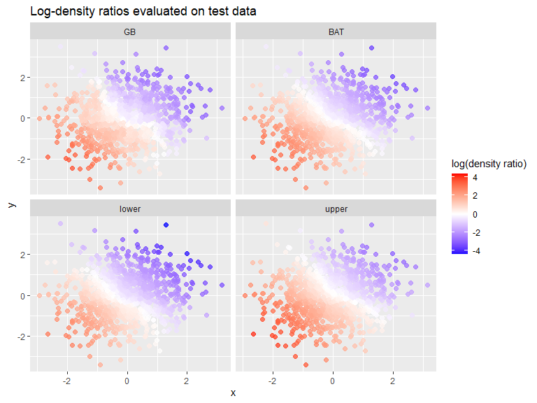
Awaya, N., Xu, Y., and Ma, L. (2025). Two-sample comparison through additive tree models for density ratios.