The goal of the BayesGP package is to efficiently
implement model-based smoothing with flexible GP priors, within a
variety of Bayesian hierarchical models.
You can install the development version of BayesGP from GitHub with:
# install.packages("devtools")
devtools::install_github("https://github.com/Bayes-GP/BayesGP/tree/development")In this example, we will use the lynx dataset as an
example, which can be accessed directly from R. Let’s load the dataset
and visualize it:
library(BayesGP)
data <- data.frame(year = seq(1821, 1934, by = 1), y = as.numeric(lynx))
data$x <- data$year - min(data$year)
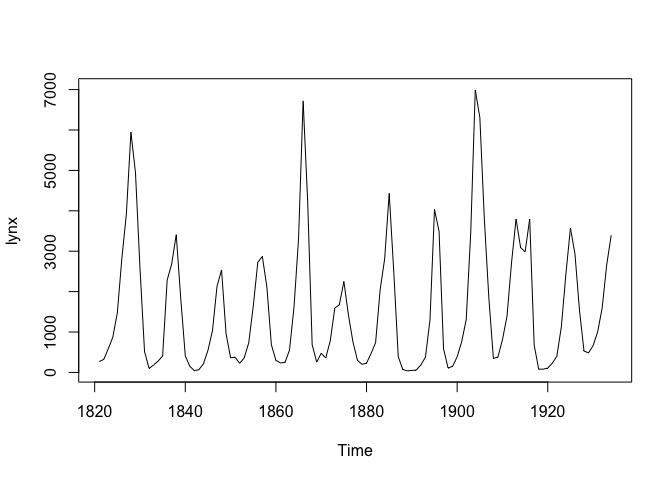
plot(lynx)
Based on a visual examination of the dataset, we can observe an obvious 10-year quasi-periodic behavior in the lynx count with evolving amplitudes over time. Therefore, we will consider fitting the following model:
\[ \begin{equation} \begin{aligned} y_i|\lambda_i &\sim \text{Poisson}(\lambda_i) ,\\ \log(\lambda_i) &= \eta_i = \beta_0 + g(x_i) + \xi_i,\\ g &\sim \text{sGP} \bigg(\alpha = \frac{2\pi}{10}, \sigma\bigg),\\ \xi_i &\sim N(0,\sigma_\xi). \end{aligned} \end{equation} \] Here, each \(y_i\) represents the lynx count, \(x_i\) represents the number of years since 1821, and \(\xi_i\) is an observation-level random intercept to account for overdispersion effect.
To specify the priors for the sGP boundary conditions and the intercept parameter, we assume independent normal priors with mean 0 and variance 1000. For the overdispersion parameter \(\sigma_\xi\), we assign an exponential prior with \(P(\sigma_\xi > 1) = 0.01\).
To determine the prior for the standard deviation parameter \(\sigma\) of the sGP, we employ the concept of predictive standard deviation (PSD). We start with an exponential prior on the 50 years PSD: \[P(\sigma(50)>1) = 0.01.\]
To make inference of the quasi-periodic seasonal effect through the
seasonal-B spline approach, we make use of the model_fit
function from BayesGP. The prior information of the sGP
component should be specified in f(.). The argument
k = 30 will setup 30 equally spaced seasonal B-spline basis
functions for the approximation. A higher value of k will
increase the approximation accuracy of the seasonal B-spline
approximation, at the cost of longer runtime.
By default, the posterior is obtained through an approximation using
the adaptive quadrature method described in the main paper. However,
exact method through MCMC sampling is also possible, by specifying
method = "MCMC" in model_fit.
mod <- model_fit(formula = y ~ f(x, model = "sgp", period = 10, k = 30,
                                 sd.prior = list(param = list(u = 1, alpha = 0.01), h = 50),
                                 boundary.prior = list(prec = 0.001)) +
                   f(year, model = "iid", sd.prior = list(param = list(u = 1, alpha = 0.01))),
                 family = "Poisson", data = data, method = "aghq")
The posterior summary of the fitted model can be examined through
summary or plot:
summary(mod)
#> Here are some posterior/prior summaries for the parameters:
#>        name median q0.025 q0.975       prior prior:P1 prior:P2
#> 1 intercept  6.687  6.508  6.868      Normal        0    1e+03
#> 2   x (PSD)  2.841  2.230  3.591 Exponential        1    1e-02
#> 3 year (SD)  0.250  0.194  0.325 Exponential        1    1e-02
#> For Normal prior, P1 is its mean and P2 is its variance.
#> For Exponential prior, prior is specified as P(theta > P1) = P2.plot(mod)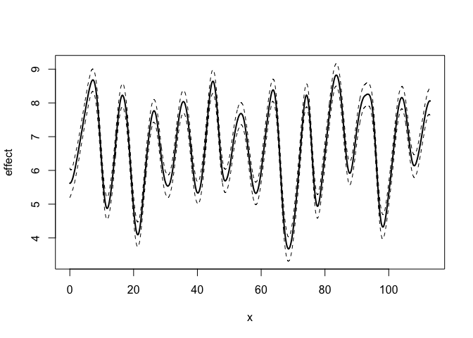
This is a basic example which shows you how to use
BayesGP to fit and analyze some models, we consider the
following data set of COVID-19 mortality in Canada, which is available
in the package:
library(BayesGP)
## basic example code
head(covid_canada)
#>         Date new_deaths        t weekdays1 weekdays2 weekdays3 weekdays4
#> 1 2020-03-01          0 591.0323        -1        -1        -1        -1
#> 2 2020-03-02          0 591.0645         1         0         0         0
#> 3 2020-03-03          0 591.0968         0         1         0         0
#> 4 2020-03-04          0 591.1290         0         0         1         0
#> 5 2020-03-05          0 591.1613         0         0         0         1
#> 6 2020-03-06          0 591.1935         0         0         0         0
#>   weekdays5 weekdays6 index
#> 1        -1        -1     1
#> 2         0         0     2
#> 3         0         0     3
#> 4         0         0     4
#> 5         0         0     5
#> 6         1         0     6
We can fit a model with \(\text{IWP}_3(\sigma)\) prior using the
function model_fit:
fit_result <- model_fit(new_deaths ~ weekdays1 + weekdays2 + weekdays3 + weekdays4 + weekdays5 + weekdays6 +
                          f(smoothing_var = t, model = "IWP", order = 3, k = 30),
                        data = covid_canada, method = "aghq", family = "Poisson")
We can take a look at the posterior summary of this model:
summary(fit_result)
#> Here are some posterior/prior summaries for the parameters:
#>        name median q0.025 q0.975       prior prior:P1 prior:P2
#> 1 intercept  3.668  3.593  3.743      Normal        0    1e+03
#> 2 weekdays1  0.093  0.070  0.117      Normal        0    1e+03
#> 3 weekdays2  0.079  0.055  0.102      Normal        0    1e+03
#> 4 weekdays3  0.127  0.103  0.150      Normal        0    1e+03
#> 5 weekdays4  0.125  0.101  0.149      Normal        0    1e+03
#> 6 weekdays5  0.050  0.025  0.074      Normal        0    1e+03
#> 7 weekdays6 -0.152 -0.178 -0.126      Normal        0    1e+03
#> 8    t (SD)  5.175  4.009  6.940 Exponential        1    5e-01
#> For Normal prior, P1 is its mean and P2 is its variance.
#> For Exponential prior, prior is specified as P(theta > P1) = P2.
We can also see the inferred function \(f\):
plot(fit_result)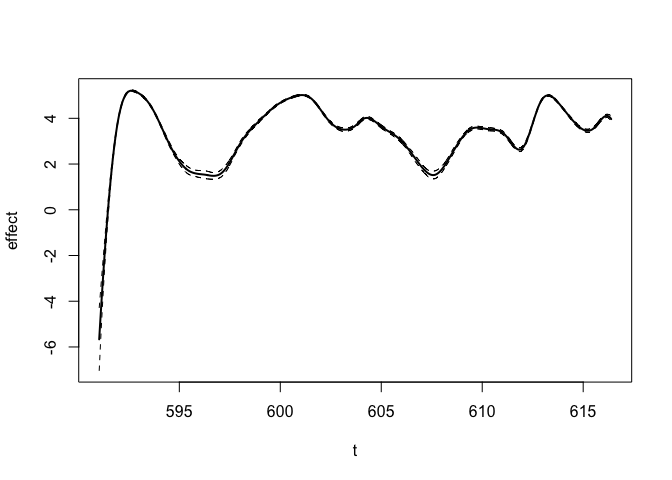
We can use the predict function to obtain the posterior
summary of \(f\) or its derivative at
new_data.
For the function \(f\):
library(tidyverse)
#> ── Attaching core tidyverse packages ──────────────────────── tidyverse 2.0.0 ──
#> ✔ dplyr     1.1.3     ✔ readr     2.1.4
#> ✔ forcats   1.0.0     ✔ stringr   1.5.0
#> ✔ ggplot2   3.5.1     ✔ tibble    3.2.1
#> ✔ lubridate 1.9.3     ✔ tidyr     1.3.0
#> ✔ purrr     1.0.2
#> ── Conflicts ────────────────────────────────────────── tidyverse_conflicts() ──
#> ✖ dplyr::filter() masks stats::filter()
#> ✖ dplyr::lag()    masks stats::lag()
#> ℹ Use the conflicted package (<http://conflicted.r-lib.org/>) to force all conflicts to become errors
predict_f <- predict(fit_result, variable = "t", newdata = data.frame(t = seq(from = 605, to = 617, by = 0.1)))
predict_f %>% ggplot(aes(x = t)) + geom_line(aes(y = mean), lty = "solid") +
  geom_line(aes(y = `q0.025`), lty = "dashed") +
  geom_line(aes(y = `q0.975`), lty = "dashed") +
  theme_classic()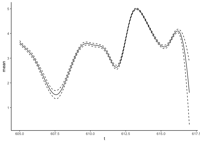
For the first derivative:
predict_f1st <- predict(fit_result, variable = "t", newdata = data.frame(t = seq(from = 605, to = 617, by = 0.1)), deriv = 1)
predict_f1st %>% ggplot(aes(x = t)) + geom_line(aes(y = mean), lty = "solid") +
  geom_line(aes(y = `q0.025`), lty = "dashed") +
  geom_line(aes(y = `q0.975`), lty = "dashed") +
  theme_classic()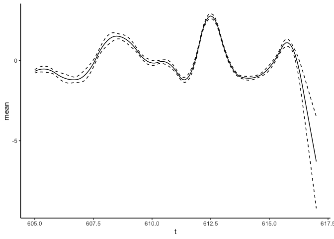
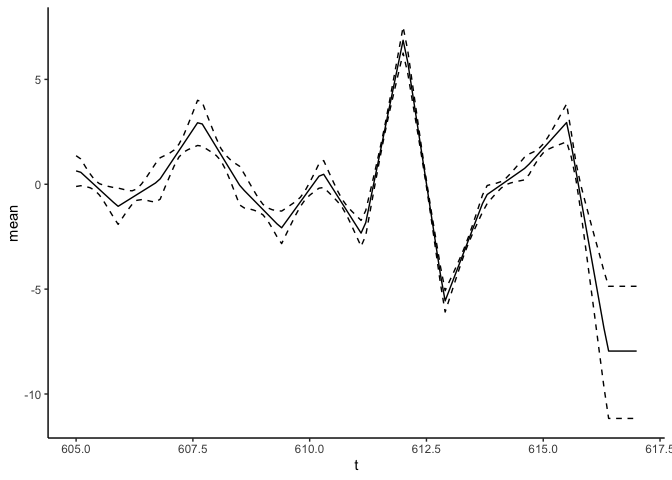
For the second derivative:
predict_f2nd <- predict(fit_result, variable = "t", newdata = data.frame(t = seq(from = 605, to = 617, by = 0.1)), deriv = 2)
predict_f2nd %>% ggplot(aes(x = t)) + geom_line(aes(y = mean), lty = "solid") +
  geom_line(aes(y = `q0.025`), lty = "dashed") +
  geom_line(aes(y = `q0.975`), lty = "dashed") +
  theme_classic()