![]()
![]()
ProbBreed employs Bayesian statistics to analyse multi-environment trials’ data, and uses its outputs to estimate the marginal and pairwise probabilities of superior performance and superior stability of the genotypes, as well as their conditional probability of superior performance. The method is thoroughly described at https://doi.org/10.1007/s00122-022-04041-y.
You can install the CRAN version of ProbBreed using the
following command:
install.packages("ProbBreed")Alternatively, you can install the development version of
ProbBreed from GitHub with:
# install.packages("devtools")
devtools::install_github("saulo-chaves/ProbBreed")library(ProbBreed)Currently, ProbBreed has nine available models
implemented in the bayes_met function. See
?bayes_met for more details. An examples using the
maize example dataset is described below:
mod = bayes_met(data = maize,
                gen = "Hybrid",
                loc = "Location",
                repl = c("Rep","Block"),
                trait = "GY",
                reg = "Region",
                year = NULL,
                res.het = TRUE,
iter = 4000, cores = 4, chain = 4)gen, loc, repl,
year and reg are all column names that contain
information on genotypes, environments (locations), replicates, years
(or seasons) and regions (or mega-environments). The maize
has no multi-year information, so year = NULL.
res.het indicates if a per-environmental residual variance
should be estimated. trait is the column in
data that contain the phenotypic observations. The other
arguments are specifications for model fitting: the number of
iterations, cores and chains. Feel free to customize these and other
options according to your necessity.
The output of this function will be an object of class
stanfit, which should be used in the extr_outs
function for further processing before computing the probabilities per
se. This function also provides some useful diagnostics. Here is how to
use it:
outs = extr_outs(model = mod,
                 probs = c(0.05, 0.95),
                 verbose = TRUE)
The object of class extr provided by this function
contains the effects’ posterior and maximum posterior, the models’
variance components and some posterior predictive checks. Here are
them:
outs$variances
#>             effect   var     sd naive.se HPD_0.05 HPD_0.95
#> 1              Rep 0.036  0.040    0.000    0.001    0.108
#> 2            Block 0.214  0.049    0.001    0.137    0.298
#> 3           Hybrid 0.217  0.075    0.001    0.118    0.353
#> 4         Location 7.995  3.864    0.043    3.773   15.124
#> 5  Hybrid:Location 0.369  0.068    0.001    0.260    0.485
#> 6           Region 4.712 18.433    0.206    0.013   17.110
#> 7    Hybrid:Region 0.056  0.041    0.000    0.002    0.130
#> 8       error_env1 0.879  0.200    0.002    0.595    1.236
#> 9       error_env2 0.945  0.257    0.003    0.593    1.418
#> 10      error_env3 1.398  0.315    0.004    0.961    1.965
#> 11      error_env4 0.591  0.147    0.002    0.388    0.862
#> 12      error_env5 1.062  0.240    0.003    0.732    1.494
#> 13      error_env6 1.453  0.327    0.004    0.980    2.039
#> 14      error_env7 0.285  0.073    0.001    0.186    0.420
#> 15      error_env8 2.000  0.476    0.005    1.311    2.847
#> 16      error_env9 0.581  0.165    0.002    0.362    0.884
#> 17     error_env10 0.628  0.150    0.002    0.423    0.905
#> 18     error_env11 1.254  0.288    0.003    0.851    1.779
#> 19     error_env12 0.456  0.116    0.001    0.296    0.670
#> 20     error_env13 0.732  0.179    0.002    0.484    1.062
#> 21     error_env14 1.834  0.401    0.004    1.264    2.556
#> 22     error_env15 0.826  0.189    0.002    0.567    1.172
#> 23     error_env16 1.813  0.422    0.005    1.221    2.584
outs$ppcheck
#>                   Diagnostics
#> p.val_max              0.3390
#> p.val_min              0.3222
#> p.val_median           0.5479
#> p.val_mean             0.5011
#> p.val_sd               0.5294
#> Eff_No_parameters    184.3898
#> WAIC2               3924.8912
#> mean_Rhat              1.0005
#> Eff_sample_size        0.8484
You can also the plot S3 method for some useful
visualizations. For e.g., the comparison between the empirical and
sampled phenotype illustrates the model’s convergence:
plot(outs)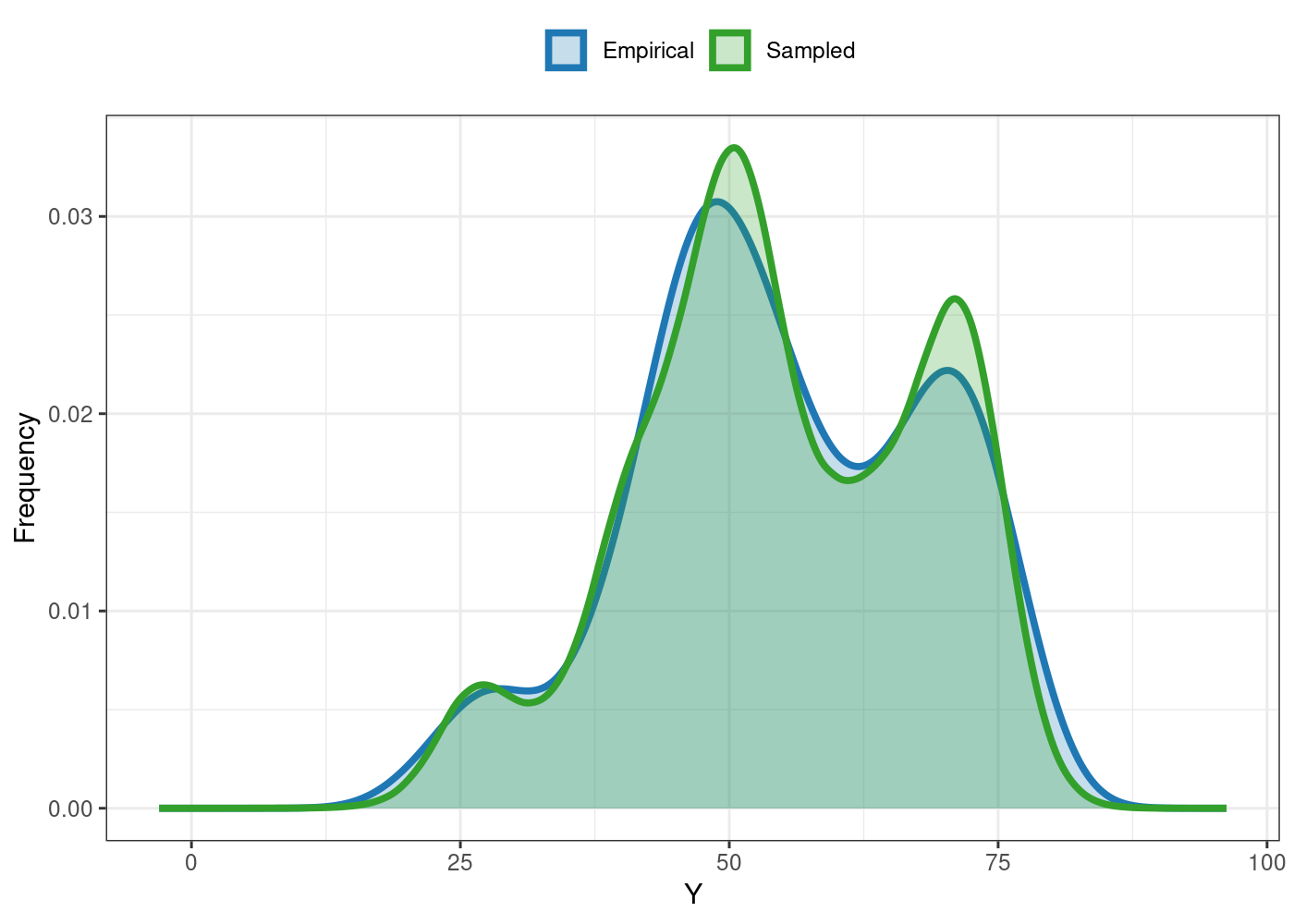
See ?plot.extr for more details and further options.
After these two steps, everything is set to compute the
probabilities. This can be done using the function
prob_sup:
A basic workflow using the available data is:
results = prob_sup(extr = outs,
                   int = .2,
                   increase = TRUE,
                   save.df = FALSE,
                   verbose = TRUE)
This function generates an object of class probsup,
which contains two lists: across and within.
As their names suggest, the across list has the
across-environments probabilities, and is suitable for a broader
recommendation. Conversely, the within results are more
appropriate to specific recommendations. For example, here are some
probability of superior performances across and within environments:
head(results$across$perfo)
#>     ID     prob
#> 36  G9 0.997500
#> 1   G1 0.920000
#> 22 G29 0.788500
#> 24 G30 0.629375
#> 5  G13 0.616250
#> 35  G8 0.569000
head(results$within$perfo$gl)
#>   gen       E1      E10      E11      E12      E13      E14      E15      E16
#> 1  G1 0.984000 0.277875 0.386375 0.434125 0.262625 0.953625 0.311625 0.972625
#> 2 G10 0.010250 0.000875 0.001750 0.002500 0.026500 0.068000 0.000125 0.043000
#> 3 G11 0.006250 0.100125 0.110625 0.004875 0.608000 0.111875 0.745375 0.094750
#> 4 G12 0.153875 0.093000 0.045125 0.058750 0.064375 0.302125 0.173250 0.569250
#> 5 G13 0.202875 0.194625 0.136375 0.134125 0.070375 0.595250 0.807125 0.068500
#> 6 G14 0.000000 0.006750 0.111375 0.156500 0.030375 0.070875 0.000375 0.023625
#>         E2       E3       E4       E5       E6       E7       E8       E9
#> 1 0.899000 0.619250 0.907125 0.522125 0.302500 0.005500 0.863875 0.385625
#> 2 0.093000 0.199250 0.001625 0.042875 0.024375 0.001750 0.000250 0.044000
#> 3 0.020625 0.031625 0.014250 0.110000 0.340375 0.017375 0.049625 0.229500
#> 4 0.413625 0.602125 0.193125 0.389125 0.430500 0.819750 0.160375 0.313000
#> 5 0.234375 0.705375 0.684750 0.606250 0.825625 0.467125 0.118750 0.537375
#> 6 0.001625 0.048000 0.122625 0.114750 0.631000 0.025000 0.037875 0.065000
The S3 method plot is also available for
probsup objects. Here are some of them:
plot(results)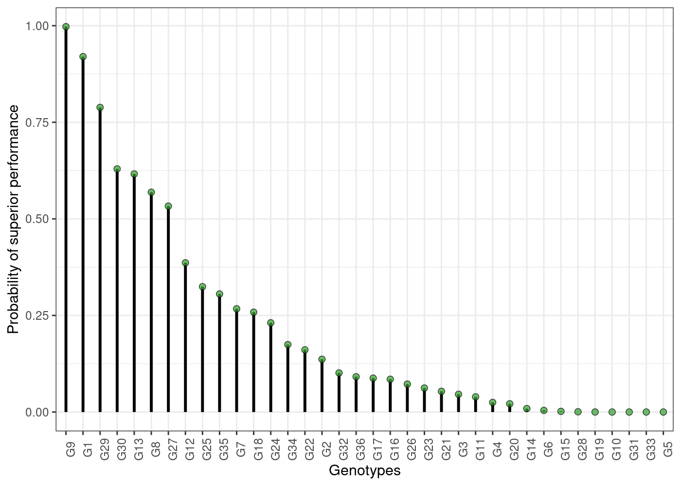
plot(results, category = "pair_perfo", level = "across")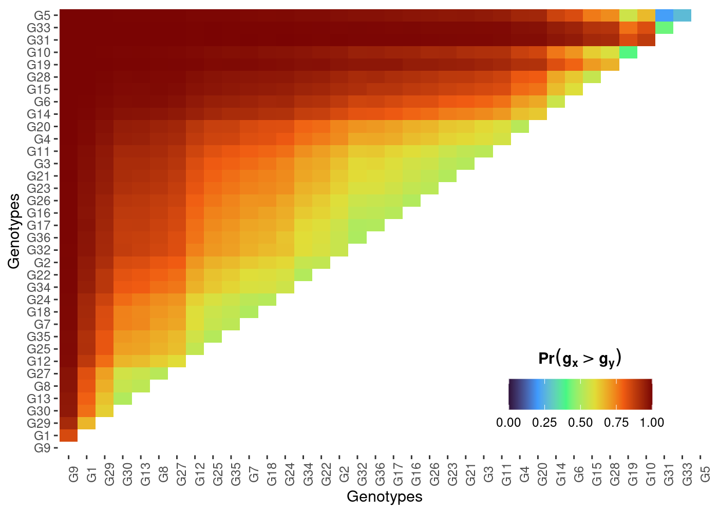
plot(results, category = "stabi")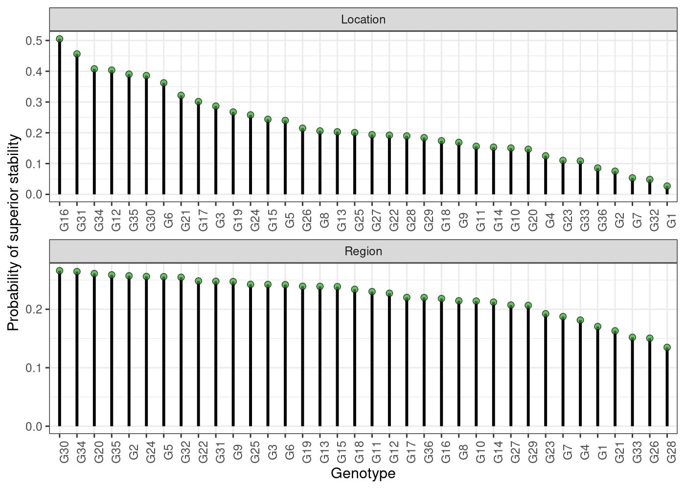
plot(results, category = "perfo", level = "within")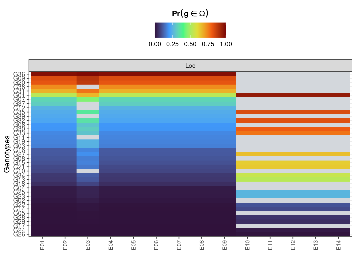
See more options at ?plot.probsup.
The estimation of these probabilities are strictly related to some key questions that constantly arises in plant breeding, like:
What is the risk of recommending a selection candidate for a target population of environments?
What is the probability of a given selection candidate having good performance if recommended to a target population of environments? And for a specific environment?
What is the probability of a given selection candidate having better performance than a cultivar check in the target population of environments? And in specific environments?
How probable is it that a given selection candidate performs similarly across environments?
What are the chances that a given selection candidate is more stable than a cultivar check in the target population of environments?
What is the probability that a given selection candidate having a superior and invariable performance across environments?
For a more detailed tutorial, see https://saulo-chaves.github.io/ProbBreed_site/.
Thank you for using ProbBreed! Please, do not forget to
cite:
citation('ProbBreed')