curves

curves is an experimental R package for plotting response curves from fitted models with ggplot2. The package is intentionally small and model-agnostic: supply a fitted model, predictor data, and, when needed, a custom prediction function.

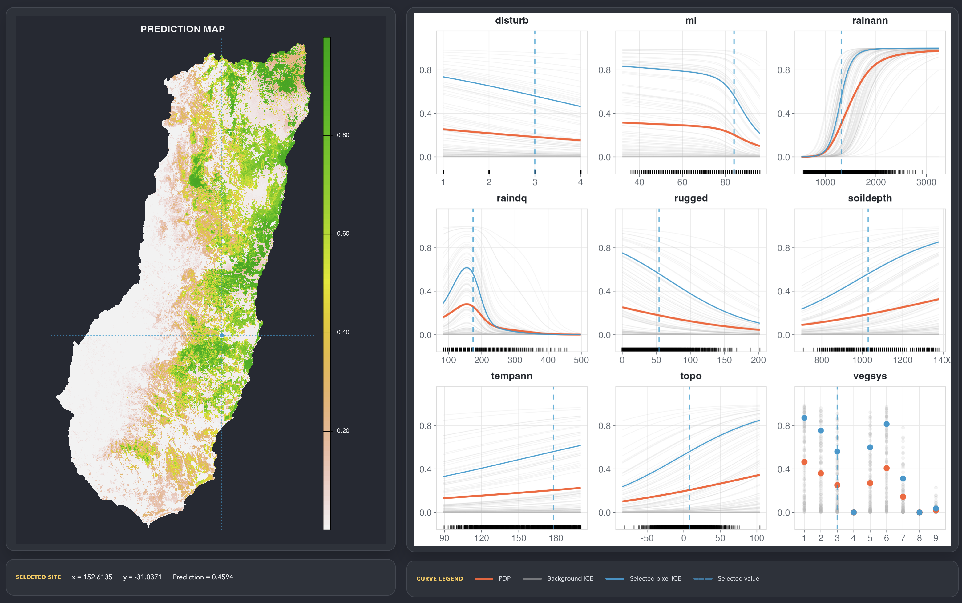
The figure above shows partial dependence curves from the included species distribution vignette.

Current package scope

The current API is centred around five exported functions:

• univariate() for one-predictor response curves with method = "profile", "pdp", "ice", "ice+pdp", or "ale".
• bivariate() for two-predictor profile, PDP, or ALE surfaces as static heatmaps, filled contours, or interactive 3D plotly surfaces.
• interactions() for ranking numeric predictor pairs by the strength of their centred second-order ALE interaction surfaces.
• multimodel() for ensemble profile, PDP, or ALE curves across multiple fitted models, with optional interval ribbons and member-model overlays.
• mapcurve() for Shiny-based exploration that links a prediction raster to response curves at clicked map cells.

A few practical details are worth calling out:

• Predictor inputs can be ordinary data frames or terra::SpatRaster objects.
• Numeric and factor predictors are supported. Univariate ALE summaries now support both numeric and factor predictors, while bivariate ALE remains limited to numeric predictor pairs.
• If predict() returns multiple columns, response can be used to choose the column to plot.
• Static plots return ggplot2 objects, so they can be styled or combined in downstream workflows.

In short, profile curves use one reference row, PDP averages predictions over sampled rows, ICE keeps those row-level curves visible, and ALE accumulates local prediction differences within the observed predictor distribution.

Installation

curves is not on CRAN. Install the development version from GitHub:

install.packages("remotes")
remotes::install_github("rvalavi/curves")

Optional packages:

• terra for raster-backed predictor inputs.
• plotly for interactive 3D surfaces.
• mgcv for the GAM ensemble example below.
• randomForest and disdat for the species distribution vignette.

Quick start

library(curves)

model <- lm(
  Sepal.Length ~ Sepal.Width + Petal.Length + Petal.Width,
  data = iris
)

predictors <- iris[, c("Sepal.Width", "Petal.Length", "Petal.Width")]

# Partial dependence curves (default)
univariate(model, predictors)

# Single-profile response curves
univariate(
  model,
  predictors,
  method = "profile"
)

# Accumulated local effects curves
univariate(model, predictors, method = "ale", n = 40)

# Bivariate response surface
bivariate(
  model,
  predictors,
  pairs = c("Sepal.Width", "Petal.Length"),
  background_n = 50,
  rug = TRUE,
  plot_type = "heatmap"
)

# Rank pairwise ALE interactions
interactions(model, predictors, n = 10)

# Plot only the strongest ALE surfaces
bivariate(model, predictors, method = "ale", top_n = 3, n = 10)

For ensemble modelling or repeated-fit comparisons, pass a list of fitted models to multimodel(). This is useful not only for formal ensembles, but also for cross-validation folds, bootstrap or bagged refits, and models fit with different background samples or closely related training sets. The models should share compatible predictors, and their predictions should be on the same response scale. If a set of models shares the same prediction interface, pass non-default prediction arguments through .... For mixed model types, supply fun as a list of wrappers, one per model. If a shared prediction function returns multiple prediction columns, either set response or provide a small wrapper through fun. Use agg, weights, interval, and show_models to control how the model curves are combined and displayed.

models <- list(
  lm(Sepal.Length ~ Sepal.Width + Petal.Length, data = iris),
  mgcv::gam(Sepal.Length ~ s(Sepal.Width) + s(Petal.Length), data = iris)
)

multimodel(
  models,
  predictors[, c("Sepal.Width", "Petal.Length")],
  background_n = 200,
  show_models = TRUE
)

Species distribution vignette

The package includes a fuller species distribution vignette built around a down-sampled random forest classifier. It demonstrates:

• presence-class response plots with response = "1"
• profile, PDP, ICE, and ALE workflows through univariate()
• bivariate profile, PDP, and ALE surfaces with an optional 3D surface

You can open it after installation with:

vignette("random-forest-species-distribution", package = "curves")

Interactive map-linked curves

mapcurve() opens a Shiny explorer that links a predicted map to fitted response curves. Clicking a raster cell marks that site’s predictor values on the curve panels, which helps compare local conditions with profile, PDP, ICE, or ALE summaries.