![]()
![]()
The goal of {migrate} is to provide users with an easy set of tools for building state transition matrices.
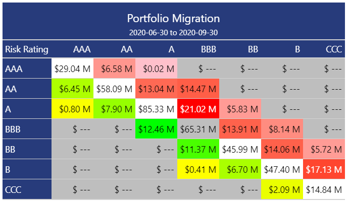
{migrate} provides an easy way to calculate absolute or percentage migration within a credit portfolio. The above image shows a typical credit migration matrix using the absolute approach; each cell in the grid represents the total balance in the portfolio at 2020-06-30 that started at the Risk Rating represented on the left-hand vertical axis and ended (at 2020-09-30) at the Risk Rating represented on the upper horizontal axis of the matrix. For example, $6.58M moved from a Risk Rating AAA at 2020-06-30 to a Risk Rating AA at 2020-09-30.
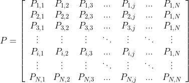
While the above, absolute, migration example is typically more of a reporting function, the percentage (or probabilistic) methodology is often more of a statistical modeling exercise, often used in credit portfolio risk management. Currently, this package only supports the simple “cohort” methodology. This estimates the probability of moving from state i to state j in a single time step, echoing a Markov process. We can visualize this in a matrix, for a credit portfolio with N unique, ordinal states:
Future development plans for this package include building functionality for the more complex duration/hazard methodology, including both the time-homogeneous and non-homogeneous implementations.
You can install the released version of {migrate} from CRAN with:
install.packages("migrate")And the development version from GitHub with:
# install.packages("devtools")
devtools::install_github("ketchbrookanalytics/migrate"){migrate} currently only handles transitions between exactly two (2)
timepoints. Under the hood, migrate() finds the earliest
& latest timepoints in the given time variable, and filters
out any observations where the time value does not match those
two periods.
migrate() identifies the desired timepoints in the
time variable by isolating the unique values and sorting. As a
result, migrate() can accommodate a variety of data types.
However, date or datetime data types are
likely the most convenient to work with.
While most data types will sort appropriately, if the time
variable is type character, it is recommended to convert to
type factor (ordered) before passing to
migrate() to ensure the time values are properly
sequenced. migrate() will throw a warning if the
time variable is type character.
If you are writing a SQL query to get data to be used with
migrate(), the query would likely look something like
this:
-- Get the *State* risk status and *Balance* dollar amount for each ID, at two distinct dates
SELECT ID, Date, State, Balance
FROM my_database
WHERE Date IN ('2020-12-31', '2021-06-30')
By default, migrate() drops observations that belong to
IDs found at a single timepoint. However, users can define a filler
state so that IDs with a single timepoint are not removed but
rather migrated from or to this filler state. This allows for
more flexible handling of such data, ensuring that no information is
lost during the migration process. Check Handle
IDs with observations at a single timepoint for more
information.
First, load the package using library()
library(migrate)The package has a built-in mock dataset, which can be loaded into the environment like so:
data("mock_credit")

head(mock_credit[order(mock_credit$customer_id), ]) # sort by 'customer_id'| customer_id | date | risk_rating | principal_balance |
|---|---|---|---|
| Customer_1001 | 2020-06-30 | A | 915000 |
| Customer_1001 | 2020-09-30 | A | 1328000 |
| Customer_1002 | 2020-06-30 | AAA | 979000 |
| Customer_1002 | 2020-09-30 | AAA | 354000 |
| Customer_1003 | 2020-06-30 | BBB | 1400000 |
| Customer_1003 | 2020-09-30 | BBB | 356000 |
Note that an important feature of the mock_credit
dataset is that there are exactly two (2) unique values in the
date column variable; if the time argument
passed to migrate() has more than two (2) unique values,
the function will throw an error.
unique(mock_credit$date)
#> [1] "2020-06-30" "2020-09-30"
To summarize the migration within the data, use the
migrate() function
migrated_df <- migrate(
  data = mock_credit,
  id = customer_id,
  time = date,
  state = risk_rating,
)
#> ℹ Migrating from 2020-06-30 to 2020-09-30
head(migrated_df)
#> # A tibble: 6 × 3
#>   risk_rating_start risk_rating_end   prop
#>   <ord>             <ord>            <dbl>
#> 1 AAA               AAA             0.774
#> 2 AAA               AA              0.194
#> 3 AAA               A               0.0323
#> 4 AAA               BBB             0
#> 5 AAA               BB              0
#> 6 AAA               B               0
To create the state transition matrix, use the
build_matrix() function
build_matrix(migrated_df)
#> ℹ Using `risk_rating_start` as the 'state_start' column variable
#> ℹ Using `risk_rating_end` as the 'state_end' column variable
#> ℹ Using `prop` as the 'metric' column variable
#>             AAA         AA          A        BBB         BB          B        CCC
#> AAA 0.774193548 0.19354839 0.03225806 0.00000000 0.00000000 0.00000000 0.00000000
#> AA  0.101123596 0.66292135 0.15730337 0.07865169 0.00000000 0.00000000 0.00000000
#> A   0.008333333 0.06666667 0.72500000 0.16666667 0.03333333 0.00000000 0.00000000
#> BBB 0.000000000 0.00000000 0.11363636 0.68181818 0.14772727 0.05681818 0.00000000
#> BB  0.000000000 0.00000000 0.00000000 0.11392405 0.63291139 0.16455696 0.08860759
#> B   0.000000000 0.00000000 0.00000000 0.01388889 0.09722222 0.62500000 0.26388889
#> CCC 0.000000000 0.00000000 0.00000000 0.00000000 0.00000000 0.14285714 0.85714286
Or, to do it all in one shot, use the |>
mock_credit |>
  migrate(
    id = customer_id,
    time = date,
    state = risk_rating,
    metric = principal_balance,
    percent = FALSE,
    verbose = FALSE
  ) |>
  build_matrix(
    state_start = risk_rating_start,
    state_end = risk_rating_end,
    metric = principal_balance
  )
#>          AAA       AA        A      BBB       BB        B      CCC
#> AAA 29042000  6575000    20000        0        0        0        0
#> AA   6445000 58095000 13045000 14467000        0        0        0
#> A     804000  7898000 85330000 21015000  5829000        0        0
#> BBB        0        0 12461000 65315000 13911000  8140000        0
#> BB         0        0        0 11374000 45986000 14057000  5723000
#> B          0        0        0   413000  6700000 47402000 17132000
#> CCC        0        0        0        0        0  2094000 14843000